Spark Shuffle Partitions Optimization

What is Spark shuffle and why do shuffle partitions matter?

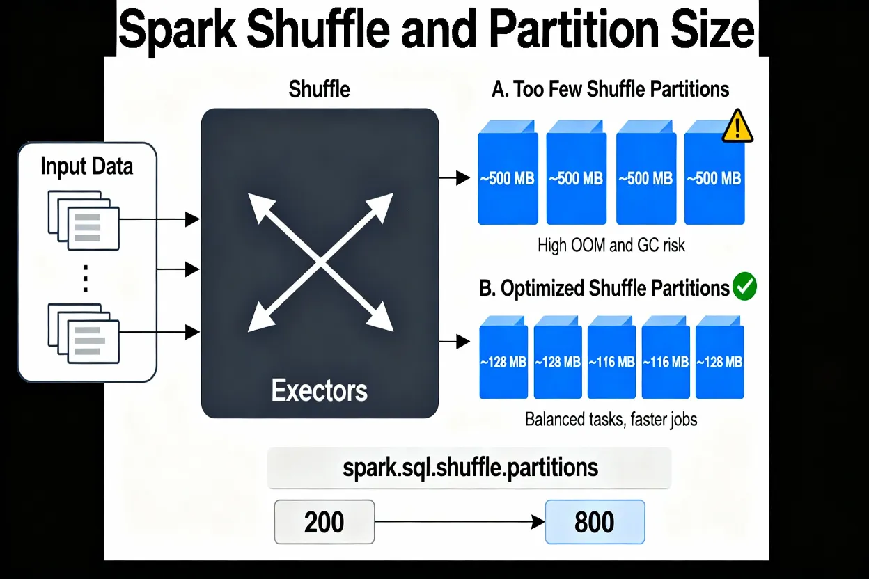
Shuffle is the step where Spark physically moves data between executors. It fires on any wide transformation — a join, groupBy, window function, or explicit repartition. During a shuffle, Spark writes intermediate data to local disk (shuffle write), then reads it back across the network into new partitions (shuffle read). The number of those new partitions is controlled by spark.sql.shuffle.partitions.

The default is 200. That was a reasonable guess in 2015 for a medium-sized cluster. In 2025, on a 100-node job processing terabytes, 200 partitions means each partition can be multiple gigabytes — the single most common cause of OOM errors and hour-long garbage collection pauses.

Reading the Spark UI: what to look for

Every optimization decision should start here. Guessing without the UI usually produces the wrong fix.

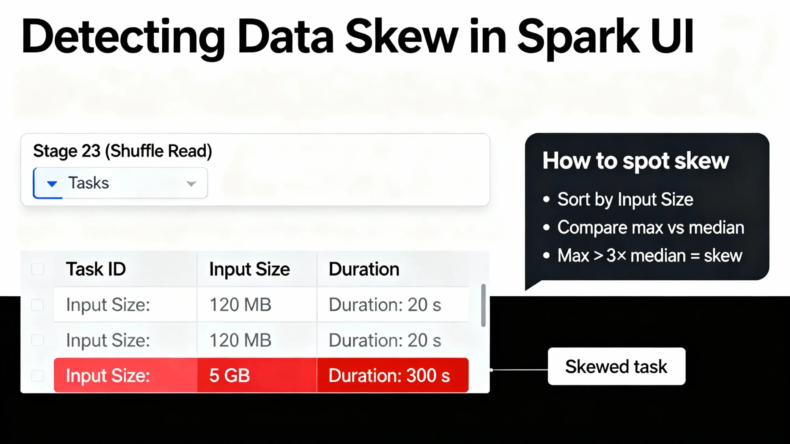
1. Open the job’s Spark UI and go to the Stages tab. Sort by Duration descending.
2. Click the slowest stage. Confirm it contains an Exchange node in the DAG (that’s the shuffle). If there’s no Exchange, the problem is elsewhere.
3. In the Tasks table, sort by Input Size / Records and then Duration. Compare the largest task to the median.
4. Skew signal: if the largest task’s input is more than 3× the median, or its runtime is more than 3× the median, you have a skew problem. AQE formally defines a skewed partition as one where size > skewedPartitionFactor × median AND size > skewedPartitionThresholdInBytes (default 256 MB).
5. Volume signal: if all tasks look similar but each one handles several hundred MB or more, you need more partitions overall — not a salting fix.

Calculating the right number of shuffle partitions

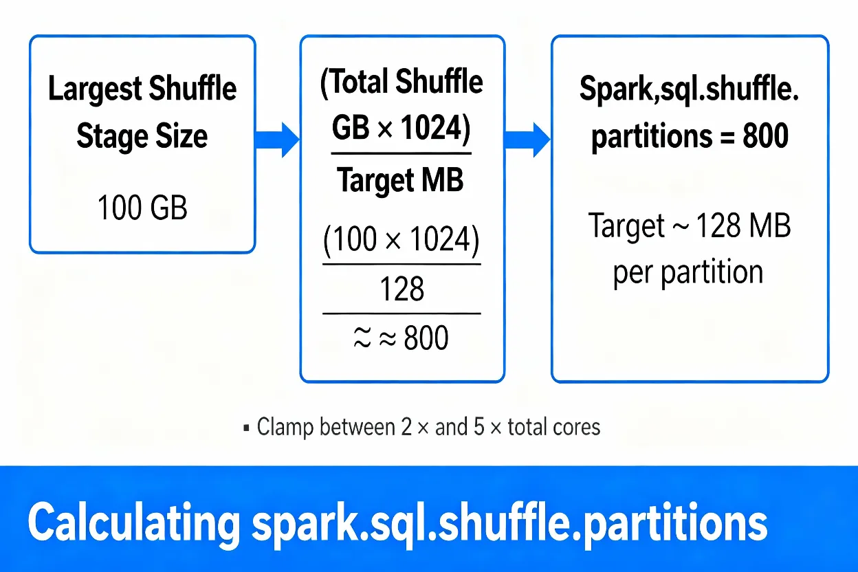
Target 100–200 MB per shuffle partition. Divide the shuffle data size of your largest stage by that target. Read the shuffle write size from the Spark UI stage summary — it’s labeled Shuffle Write.

# Read shuffle_write_gb from the Spark UI → Stage Summary → Shuffle Write
shuffle_write_gb  = 100    # e.g., 100 GB largest shuffle stage
target_mb         = 128    # target partition size — keep under 200 MB

ideal_partitions  = int((shuffle_write_gb * 1024) / target_mb)
# 100 × 1024 / 128 = 800 partitions

# Sanity checks:
# ✓ Result should be ≥ 2–5 × (number of available cluster cores)
# ✓ Each partition should stay below ~200 MB to avoid GC pressure
# ✗ Don't exceed ~5000–8000 — task scheduling overhead wins at extreme counts

# Bad: 100 GB ÷ 200 partitions = ~512 MB each → OOM likely
# Good: 100 GB ÷ 800 partitions = ~128 MB each → balanced

Setting the config — PySpark, Scala, and the key AQE knobs

Set spark.sql.shuffle.partitions early in your notebook or job script — before any wide transformation. In Databricks cluster settings you can also set it as a cluster default, but notebook-level config always takes precedence.

# 1. Set initial partition count based on your largest shuffle stage
spark.conf.set("spark.sql.shuffle.partitions", "800")

# 2. Enable AQE (default on in Databricks 7.3+ and OSS Spark 3.2+)
spark.conf.set("spark.sql.adaptive.enabled", "true")

# 3. AQE advisory partition size — how large a coalesced partition should be
spark.conf.set("spark.sql.adaptive.advisoryPartitionSizeInBytes", "134217728")  # 128 MB

# 4. Skew join handling (enabled by default when AQE is on)
spark.conf.set("spark.sql.adaptive.skewJoin.enabled", "true")

# 5. Local shuffle reader — prefer local executors for shuffle reads
spark.conf.set("spark.sql.adaptive.localShuffleReader.enabled", "true")

# Then run your heavy operations
df_result = df1.join(df2, "user_id") \
               .groupBy("country") \
               .agg(F.sum("revenue").alias("total"))

spark.conf.set("spark.sql.shuffle.partitions", "800")
spark.conf.set("spark.sql.adaptive.enabled", "true")
spark.conf.set("spark.sql.adaptive.advisoryPartitionSizeInBytes", "134217728")

val dfResult = df1.join(df2, Seq("user_id"))
                  .groupBy("country")
                  .agg(sum("revenue").alias("total"))

What AQE fixes — and where it can’t help

AQE is Spark’s runtime re-optimizer. It fires at shuffle boundaries where real statistics become available, and uses those statistics to make better decisions than the static plan could. It has four features:

1. Dynamic partition coalescing: merges adjacent small shuffle partitions into larger ones, so a job with 2,000 initial partitions may finish with 80 actual tasks.
2. Dynamic sort-merge join → broadcast hash join: if a filtered table turns out to be small enough to broadcast after the shuffle, AQE promotes the join strategy mid-execution, avoiding a second sort-merge phase.
3. Skew join handling: splits and optionally replicates skewed partitions so the hot-key task is processed by multiple tasks in parallel instead of one overwhelmed executor.
4. Empty relation propagation: if a join side is empty (e.g., a filter returns zero rows), AQE short-circuits the entire join branch rather than executing it.

Spark 4.0 (released May 2025, Databricks Runtime 17.0 June 2025) refines AQE further, with internal benchmarks showing complex queries running up to 30% faster than Spark 3.x and up to 3× faster than Spark 2.x — primarily from improved partition coalescing and join strategy switching.

Join strategy decision — in order of preference

Choosing the right join strategy can eliminate shuffle entirely. Tuning spark.sql.shuffle.partitions only helps if you’re already on the right strategy. Work top-down through this hierarchy for every expensive join:

Storage Partition Join (SPJ): no shuffle, no config to tune

Storage Partition Join (Spark 3.3+, matured in 3.4) exploits the storage layout of DataSource V2 tables — Apache Iceberg, Delta Lake, Apache Hudi — to skip the shuffle phase of a join entirely. If both tables are partitioned on the same column with the same partition function, Spark can co-locate matching data without moving it. The Spark UI shows no Exchange node in the physical plan when SPJ is active.

SPJ generalizes Bucket Joins (which work only for bucketed Hive tables) to any DataSource V2 table that reports its partitioning. At Expedia Group’s scale, enabling SPJ on co-partitioned Iceberg tables eliminated the shuffle and produced benchmark speedups that justified restructuring their table layouts specifically for it.

# Both tables must be partitioned on the same column with matching partition specs
# Example: both tables partitioned by 'region' or bucket(8, 'customer_id')

spark.conf.set("spark.sql.sources.v2.bucketing.enabled", "true")
spark.conf.set("spark.sql.sources.v2.bucketing.pushPartValues.enabled", "true")
spark.conf.set("spark.sql.iceberg.planning.preserve-data-grouping", "true")
spark.conf.set("spark.sql.requireAllClusterKeysForCoPartition", "false")
spark.conf.set("spark.sql.sources.v2.bucketing.partiallyClusteredDistribution.enabled", "true")

# Verify SPJ is working: no Exchange node should appear
df_orders.join(df_customers, "region").explain("FORMATTED")
# If Exchange is absent → SPJ is active. If Exchange appears → co-partitioning mismatch.

Salting: when AQE skew handling isn’t enough

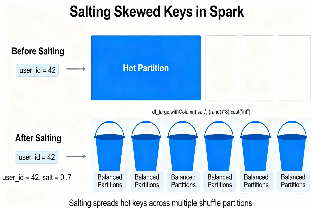
AQE’s skew join feature splits large partitions at runtime, but it works within the existing data distribution — it can’t split a partition whose entire content is rows with a single key value. If 30% of your fact table has country = 'US', AQE can split the task but Spark still needs to re-replicate the matching dimension rows to all split tasks, which adds its own overhead. Past roughly 5–10× skew on a single key, manual salting gives cleaner results.

from pyspark.sql import functions as F

skewed_col  = "user_id"
n_buckets   = 8       # spread hot keys across 8 sub-partitions

# Large (skewed) side: append a random salt column
df_large_salted = df_large.withColumn(
    "salt",
    (F.rand() * n_buckets).cast("int")
)

# Small side: cross-join with 0..n_buckets-1 so every salt value has a match
df_small_expanded = df_small.crossJoin(
    spark.range(n_buckets).toDF("salt")
)

# Join on original key + salt
df_joined = df_large_salted.join(
    df_small_expanded,
    on=[skewed_col, "salt"],
    how="inner"
)

# Aggregate and drop salt — result is identical to the unsalted join
df_result = df_joined.groupBy(skewed_col).agg(
    F.sum("metric").alias("metric_sum")
)

Preventing OutOfMemory errors from shuffle

OOM during a shuffle stage almost always means one or more partitions don’t fit in executor memory. The checklist below covers all common causes — work through it in order rather than just raising spark.executor.memory first.

• Raise spark.sql.shuffle.partitions so each partition targets 100–200 MB. Check the Spark UI to confirm task sizes after the change.
• If skewed keys drive the OOM, AQE skew join handling is the first remedy. If AQE doesn’t fully fix it (check whether isSkew=true appears in the query plan), add salting for the hottest keys.
• Audit your caching. df.cache() or df.persist() during a shuffle-heavy pipeline competes with shuffle buffers for executor memory. Unpersist DataFrames that are no longer needed with df.unpersist().
• Don’t call coalesce() before a heavy join. coalesce reduces partition count without shuffling, which can create very large input partitions that then explode during the join’s shuffle. Use repartition() to rebalance, and save coalesce() for after the join when you want fewer output files.
• Check the Spark event log for GC metrics. If GC time is >10% of task time, the JVM is struggling with memory — reducing partition size or switching to Kryo serialization (spark.serializer=org.apache.spark.serializer.KryoSerializer) helps.

Databricks and Microsoft Fabric: what’s different

Databricks

AQE is on by default from Databricks Runtime 7.3 and has been progressively improved. Databricks Runtime 17.0 (June 2025, Spark 4.0) brings the latest AQE refinements including improved SPJ support (SPARK-49839: SPJ now skips shuffles for sorts too), enhanced partition coalescing, and internal benchmarks of 20–50% speedups on complex workloads vs Spark 3.x.

The autoBroadcastJoinThreshold in Databricks is higher than the 10 MB OSS default — Databricks manages this dynamically based on cluster memory. The Photon engine (enabled by default on many compute types from DBR 9.1 LTS+) accelerates scan-heavy and aggregation workloads independently of shuffle tuning, so combine both.

Set cluster-level config in the cluster’s Spark Config field for job-wide defaults. Use notebook-level spark.conf.set() to override for specific heavy stages.

Microsoft Fabric

Fabric Spark notebooks honor all the same configuration parameters. Use spark.conf.set() at the notebook level. The Fabric Spark UI exposes the same Stages/Tasks view for diagnosing skew and partition sizes — the diagnostic process is identical to the Spark UI steps above.

Combine shuffle tuning with Fabric-specific lakehouse design: Delta table OPTIMIZE (which compacts small files and applies Z-ordering) reduces the volume of data scanned before the shuffle, which means the shuffle itself starts with less data. See the Fabric Lakehouse Tutorial for the full table optimization workflow.

FAQ -Spark Shuffle Partitions Optimization