Transform Data Using Notebooks in Microsoft Fabric

Complete 2026 guide to transform data using notebooks. Master production patterns, Delta Lake merge operations, performance optimization, and real-world recipes with official Microsoft best practices.

Updated January 2026 20–25 min read Production-Ready 25+ Code Examples

What does it mean to Transform Data Using Notebooks?

To transform data using notebooks in Microsoft Fabric means utilizing an interactive coding environment (supporting PySpark, Spark SQL, and Scala) to clean, aggregate, and restructure data stored in OneLake. Unlike visual dataflows, notebooks offer full programmatic control, enabling complex logic, machine learning integration, and high-performance processing of large-scale datasets (TB+) using distributed Apache Spark clusters.

Why Transform Data Using Notebooks in Fabric

Transform data using notebooks is the gold standard for data engineering in Microsoft Fabric. Unlike Dataflow Gen2 (visual, low-code) or SQL Warehouse (static queries), notebooks provide:

Full Code Control

Write reproducible PySpark, Spark SQL, or Scala transformations with complete version history.

Spark Power

Distribute processing across clusters. Handle MB to TB+ datasets with parallel execution.

Delta Lake Native

Read/write ACID-compliant Delta tables. Merge, upsert, and optimize with ease.

Pipeline Integration

Orchestrate with Data Pipelines. Schedule, parameterize, and monitor at scale.

Transform Data Using Notebooks vs. Alternatives

ToolBest ForSkill LevelScaleCost
Dataflow Gen2Visual, low-code mapping & joinsPower Query knowledgeSmall–Medium (GB)High (visuals tax)
SQL WarehouseStatic SQL queries, aggregationsSQL expertiseLarge (TB+)Low (optimized)
Spark NotebooksComplex logic, feature engineering, MLPython/Scala + SparkMedium–Very Large (TB+)Low–Medium (optimizable)
Community Insight: Reddit users report 90% cost savings when migrating from Dataflow Gen2 to notebooks for large-scale transformations. Notebooks are the most cost-efficient way to transform data using notebooks at enterprise scale.

Quick Start: Transform Data Using Notebooks

Prerequisites

  • Required Fabric Capacity: F2 or higher
  • Required Workspace Role: Admin or Member
  • Required Lakehouse: Fabric Lakehouse as destination
  • Recommended Git Knowledge: For version control

Step 1: Create & Attach Notebook

1

Open Workspace

Navigate to your Fabric workspace. Ensure you have Admin or Member permissions.

2

Create Notebook

Click + New ItemNotebook. Choose default language (PySpark recommended).

3

Attach Lakehouse

In ribbon: AddLakehouse. Select your destination (or create new).

4

Write First Cell

Read a Delta table and inspect schema.

Step 2: Read Delta Tables

# Read from Lakehouse attached table df = spark.read.format(“delta”).table(“Lakehouse.schema.sales_raw”)# Inspect df.printSchema() # Column names & types df.show(5) # First 5 rows print(f”Rows: {df.count()}”)

Step 3: Transform & Clean

from pyspark.sql.functions import col, when, isnan, current_timestamp# Data quality checks bad_rows = df.filter( (col(“amount”).isNull()) | (col(“amount”) < 0) )# Write errors to table for review if bad_rows.count() > 0: bad_rows.write.format(“delta”).mode(“append”).saveAsTable(“Lakehouse.errors.quality_issues”)# Clean data df_clean = df.filter( (col(“amount”).isNotNull()) & (col(“amount”) >= 0) ).dropDuplicates([“order_id”]) \ .withColumn(“processed_date”, current_timestamp())print(f”✅ {df_clean.count()} rows passed validation”)

Step 4: Write Curated Delta Table

# Merge to curated table (idempotent upsert) from delta.tables import DeltaTabletarget = DeltaTable.forName(spark, “Lakehouse.curated.sales”) target.alias(“tgt”).merge( df_clean.alias(“src”), “tgt.order_id = src.order_id” ).whenMatchedUpdateAll().whenNotMatchedInsertAll().execute()print(f”✅ Merge complete: {df_clean.count()} rows”)
First Success: You’ve written your first transform data using notebooks pipeline! Now scale it: add error handling, schedule via pipelines, and optimize performance.

5 Production Patterns to Transform Data Using Notebooks

Battle-tested patterns for reliable, production-safe data transformations.

Pattern 1: Schema Enforcement & Data Quality Gates

Intent: Prevent silent failures due to schema drift. Explicit type casting and anomaly capture.

from pyspark.sql.types import StructType, StructField, IntegerType, DoubleType, StringType from pyspark.sql.functions import col, when, isnan, isnull# Define expected schema upfront expected_schema = StructType([ StructField(“order_id”, IntegerType(), False), StructField(“amount”, DoubleType(), False), StructField(“product”, StringType(), True) ])# Read with schema enforcement df = spark.read.schema(expected_schema).option(“mode”, “FAILFAST”).csv(“/path/to/input”)# Quality gates bad_rows = df.filter( (col(“amount”).isNull()) | (col(“amount”) < 0) | (isnan(col("amount"))) )if bad_rows.count() > 0: bad_rows.withColumn( “error_reason”, when(col(“amount”).isNull(), “null_amount”) .when(col(“amount”) < 0, "negative_amount") .otherwise("nan_amount") ).write.format("delta").mode("append").saveAsTable("Lakehouse.errors.quality_issues")df_clean = df.filter((col("amount").isNotNull()) & (col("amount") >= 0)) print(f”✅ {df_clean.count()} rows passed quality checks”)

Pattern 2: Idempotent Merges with Delta MERGE

Intent: Make notebooks safe to rerun without duplication. Delta MERGE ensures atomicity.

from delta.tables import DeltaTable from pyspark.sql.functions import col, current_timestamp# Staged incremental data staged = spark.read.format(“delta”).table(“Lakehouse.staging.sales_incremental”)target = DeltaTable.forName(spark, “Lakehouse.curated.sales”)# MERGE: update if exists, insert if new merge_result = (target.alias(“tgt”) .merge(staged.alias(“src”), “tgt.order_id = src.order_id”) .whenMatchedUpdateAll() .whenNotMatchedInsertAll() .execute() )print(f”Merge completed: {merge_result} rows affected”)# Advanced: CDC with timestamp checks (only update if source is newer) merge_cdc = (target.alias(“tgt”) .merge(staged.alias(“src”), “tgt.order_id = src.order_id”) .whenMatchedUpdate( condition=”src.modified_date > tgt.modified_date”, set={“tgt.amount”: “src.amount”, “tgt.status”: “src.status”} ) .whenNotMatchedInsertAll() .execute() )

Pattern 3: Window Functions for Time-Series Features

from pyspark.sql.window import Window from pyspark.sql.functions import avg, sum, row_number, lag, col# Rolling 7-day average sales_window = Window.partitionBy(“product”).orderBy(“date”).rowsBetween(-6, 0) df_features = df.withColumn( “rolling_avg_7day”, avg(“sales”).over(sales_window) )# Year-over-year comparison yoy_window = Window.partitionBy(“product”).orderBy(“date”) df_features = df_features.withColumn( “prior_year_sales”, lag(“sales”, 365).over(yoy_window) )# Ranking products by sales rank_window = Window.partitionBy(“date”).orderBy(col(“sales”).desc()) df_features = df_features.withColumn( “product_rank”, row_number().over(rank_window) )df_features.display()

Pattern 4: Feature Engineering & Versioning

from pyspark.sql.functions import sum, avg, count, max, datediff, current_date, when, lit# Customer-level aggregations features_v2 = transactions.groupBy(“customer_id”).agg( sum(“amount”).alias(“total_spend”), avg(“amount”).alias(“avg_transaction”), count(“*”).alias(“transaction_count”), max(“date”).alias(“last_purchase_date”) ).withColumn( “days_since_purchase”, datediff(current_date(), col(“last_purchase_date”)) ).withColumn( “is_high_value”, when(col(“total_spend”) > 10000, 1).otherwise(0) ).withColumn( “feature_version”, lit(“v2”) )# Write with partition for incremental refresh features_v2.write.format(“delta”).mode(“overwrite”) \ .option(“partitionBy”, “feature_date”) \ .option(“optimizeWrite”, “true”) \ .saveAsTable(“Lakehouse.features.customer_features_v2″)print(f”✅ Feature table: {features_v2.count()} customers, v2”)

Pattern 5: Incremental Ingestion with Partition Pruning

from datetime import datetime, timedelta from pyspark.sql.functions import current_date# Process only yesterday’s data run_date = datetime.now() – timedelta(days=1) source_path = f”/mnt/raw/sales/{run_date.date()}/”df_incremental = spark.read.format(“csv”).option(“header”, “true”).load(source_path)# Dedupe & normalize df_clean = df_incremental.dropDuplicates([“order_id”]) \ .withColumn(“ingestion_date”, current_date())# Idempotent merge target = DeltaTable.forName(spark, “Lakehouse.curated.sales”) target.alias(“tgt”).merge( df_clean.alias(“src”), “tgt.order_id = src.order_id” ).whenMatchedUpdateAll().whenNotMatchedInsertAll().execute()print(f”✅ Incremental load: {run_date.date()}”)

Transform Data Using Notebooks: Performance Optimization

When you transform data using notebooks at scale, optimize for speed and cost. Focus on reducing data movement (shuffle).

Top 5 Performance Levers

1. Partition Strategically

Split tables into 0.5–2 GB partitions by date or business keys. Massive read speedup for range filters.

2. Filter Early

Push predicates before joins. Predicate pushdown reduces data scanned by 50–99%.

3. Broadcast Dimensions

Broadcast small tables (<100 MB) to avoid shuffle in joins. Dramatic speed improvement.

4. Z-Order / Liquid Cluster

Multi-dimensional clustering for targeted queries. 50–80% read time reduction for common filters.

5. Monitor Spark UI

Profile shuffle, task count, and duration. Identify bottlenecks and tune accordingly.

Detailed: Partitioning for Transform Data Using Notebooks

# Bad: no partitioning (single large file, slow reads) df.write.format(“delta”).mode(“overwrite”).saveAsTable(“table”)# Good: single partition by date df.write.format(“delta”).mode(“overwrite”) \ .option(“partitionBy”, “date”) \ .saveAsTable(“table”)# Better: multi-level + optimize df.write.format(“delta”).mode(“overwrite”) \ .option(“partitionBy”, “year,month”) \ .option(“optimizeWrite”, “true”) \ .saveAsTable(“table”)# Best: Liquid Clustering (auto-adaptive, Spark 3.5+) df.write.format(“delta”).mode(“overwrite”) \ .option(“clusteringColumns”, “customer_id,date”) \ .option(“optimizeWrite”, “true”) \ .saveAsTable(“table”)# Rule of thumb: Each partition should be 0.5–2 GB # Too small → many small files (slow reads) # Too large → poor parallelism

Broadcast Joins for Transform Data Using Notebooks

from pyspark.sql.functions import broadcast# Bad: large shuffle if dim table is big result = sales_df.join(dim_product_df, “product_id”)# Good: broadcast small dimension to all workers result = sales_df.join(broadcast(dim_product_df), “product_id”)# Rule: If one table < 100 MB and other > 10 GB, ALWAYS broadcast small one # Can reduce shuffle by 10x or more

Monitor with Spark UI

After running a cell, click Spark application in ribbon → open Spark UI:

  • Stages tab: Which stage took longest? Look for shuffle indicators.
  • Shuffle read/write: If shuffle > 10× input data size, investigate join/agg.
  • Tasks: How many ran in parallel? More = better parallelism.
Watch Out: Shuffle > 50GB for a 10GB input? Likely cartesian product or data skew. Add more partitions or pre-filter to fix.

Notebook UI/UX Best Practices When Transform Data Using Notebooks

Production-grade notebooks are readable, maintainable, and collaborative. Apply these patterns:

1. Header Block with Full Documentation

# ============================================================================ # NOTEBOOK: sales_transform_prod # PURPOSE: Ingest daily sales CSV, dedupe, validate, merge to curated # INPUTS: # – Raw: /mnt/raw/sales/{run_date}/*.csv # – Target: Lakehouse.curated.sales # OUTPUTS: # – Lakehouse.curated.sales (upserted) # – Lakehouse.errors.sales_quality (anomalies) # PARAMETERS: run_date (default: yesterday), environment (dev/test/prod) # SCHEDULED: Daily @ 2 AM UTC via Data Pipeline “Daily Sales ETL” # OWNER: data-engineering@company.com # LAST UPDATED: 2025-01-20 # ============================================================================from datetime import datetime, timedelta from pyspark.sql.functions import *print(f”🚀 Starting: transform data using notebooks pipeline”)

2. Centralized Configuration Cell

# ============================================================================ # CONFIGURATION # ============================================================================RUN_DATE = dbutils.widgets.get(“run_date”, str((datetime.now() – timedelta(days=1)).date())) ENVIRONMENT = dbutils.widgets.get(“environment”, “prod”)if ENVIRONMENT == “prod”: SOURCE_PATH = “abfss://workspace@prodstorage.dfs.core.windows.net/raw/sales” CURATED_TABLE = “Lakehouse.curated.sales” else: SOURCE_PATH = “abfss://workspace@devstorage.dfs.core.windows.net/raw/sales” CURATED_TABLE = “Lakehouse_Dev.curated.sales”spark.conf.set(“spark.sql.shuffle.partitions”, “200”) spark.conf.set(“spark.databricks.delta.optimizeWrite.enabled”, “true”)print(f”Config: RUN_DATE={RUN_DATE}, ENV={ENVIRONMENT}, TARGET={CURATED_TABLE}”)

3. Rich Visualizations & Interactivity

# Use display() instead of show() for rich HTML output result_df.display() # Rich table with filtering, sorting# Matplotlib plotting import matplotlib.pyplot as plt result_df.toPandas().plot(kind=’bar’, figsize=(10,6)) plt.title(“Sales by Region”) plt.show()

4. Error Handling & Logging

import logginglogger = logging.getLogger(“sales_transform”) logger.setLevel(logging.INFO)try: print(“📥 Loading data…”) df_raw = spark.read.option(“header”, “true”).csv(f”{SOURCE_PATH}/{RUN_DATE}/”) logger.info(f”Loaded {df_raw.count()} rows”) except Exception as e: logger.error(f”❌ Load failed: {str(e)}”) raise

Orchestration: Transform Data Using Notebooks at Scale

Interactive development is great; production reliability requires Data Pipelines and CI/CD.

Step 1: Parameterize Your Notebook

# Define parameters users can override at runtime dbutils.widgets.text(“run_date”, str((datetime.now() – timedelta(days=1)).date()), “Run Date”) dbutils.widgets.dropdown(“environment”, “prod”, [“dev”, “test”, “prod”], “Environment”)RUN_DATE = dbutils.widgets.get(“run_date”) ENVIRONMENT = dbutils.widgets.get(“environment”)

Step 2: Add to Data Pipeline

  1. Create new Data Pipeline in workspace.
  2. Drag Notebook activity onto canvas.
  3. In Settings, select your notebook and pass parameters via pipeline variables.
  4. Add downstream steps (copy, other notebooks) to build workflow.

Step 3: Schedule & Monitor

  1. Click Schedule in pipeline ribbon.
  2. Set recurrence (daily, hourly, weekly).
  3. Configure alerts (email on failure, retry policy, timeout).
  4. Monitor from Monitor hubCapacity metrics.

Step 4: CI/CD & Version Control

Store notebooks in Git (Azure Repos, GitHub) and use Fabric CI/CD best practices:

# Notebook structure in Git data-fabric-project/ ├── notebooks/ │ ├── sales_transform.py │ ├── customer_features.py │ └── data_quality_checks.py ├── tests/ │ ├── test_sales_transform.py ├── configs/ │ └── pipeline_params.json └── README.md
Production Readiness: Parameterized notebooks + pipelines + Git = reliable, auditable data engineering. This is the Fabric standard for enterprise deployments.

Security & Governance When Transform Data Using Notebooks

Three-Layer RBAC in Fabric

LayerControlExample
WorkspaceAdmin/Member/Viewer rolesOnly engineers are Members. Analysts are Viewers.
LakehouseRow-level security (RLS) + column maskingNA managers see only NA data. SSNs are masked.
ExecutionService principal / user identityNotebook runs under your Entra ID; inherits Lakehouse permissions.

Data Masking for PII

from pyspark.sql.functions import col, when, substring, hash# Mask SSN: show only last 4 digits df_masked = df.withColumn( “ssn_masked”, when(col(“ssn”).isNotNull(), concat(lit(“XXX-XX-“), substring(col(“ssn”), 8, 4))) .otherwise(None) ).drop(“ssn”)# Hash email for anonymization df_masked = df_masked.withColumn( “email_hash”, hash(col(“email”)) ).drop(“email”)# Verify no PII remains assert len([c for c in df_masked.columns if c in [“ssn”, “email”, “phone”]]) == 0, “PII leaked!”

Audit Logging & Lineage

Microsoft Purview integrates with Fabric to track:

  • Who accessed what data and when
  • What transformations ran
  • Data lineage (notebook → Delta table)

Enable Purview integration and automatically capture lineage for compliance audits.

Real-World Recipes: Transform Data Using Notebooks

Recipe 1: Daily Incremental Sales Load + Quality Checks

Scenario: CSV files arrive daily. Load, dedupe, validate, and upsert to curated Delta table.

from datetime import datetime, timedelta from pyspark.sql.functions import * from delta.tables import DeltaTableRUN_DATE = datetime.now() – timedelta(days=1) SOURCE_PATH = f”abfss://raw/sales/{RUN_DATE.date()}/” CURATED_TABLE = “Lakehouse.curated.sales”print(f”🚀 Daily sales load: {RUN_DATE.date()}”)# 1. READ df_raw = spark.read.option(“header”, “true”).csv(SOURCE_PATH) print(f”Loaded {df_raw.count()} raw rows”)# 2. QUALITY CHECKS bad_rows = df_raw.filter((col(“order_id”).isNull()) | (col(“amount”) < 0)) if bad_rows.count() > 0: bad_rows.write.format(“delta”).mode(“append”).saveAsTable(“Lakehouse.errors.sales_quality”)# 3. CLEAN & ENRICH df_clean = df_raw.filter( (col(“order_id”).isNotNull()) & (col(“amount”) >= 0) ).dropDuplicates([“order_id”]) \ .withColumn(“ingestion_date”, lit(RUN_DATE.date())) \ .withColumn(“ingestion_ts”, current_timestamp())# 4. MERGE (idempotent) target = DeltaTable.forName(spark, CURATED_TABLE) target.alias(“tgt”).merge( df_clean.alias(“src”), “tgt.order_id = src.order_id” ).whenMatchedUpdateAll().whenNotMatchedInsertAll().execute()print(f”✅ Merged {df_clean.count()} rows for {RUN_DATE.date()}”)

Recipe 2: Customer Feature Engineering for ML

Scenario: Build versioned feature table from transaction history for ML training.

from pyspark.sql.functions import * from pyspark.sql.window import Window# Load transaction data transactions = spark.read.format(“delta”).table(“Lakehouse.curated.sales”)# 1. AGGREGATIONS customer_agg = transactions.groupBy(“customer_id”).agg( count(“*”).alias(“transaction_count”), sum(“amount”).alias(“total_spend”), avg(“amount”).alias(“avg_transaction”), max(“date”).alias(“last_purchase_date”) )# 2. TEMPORAL FEATURES customer_agg = customer_agg.withColumn( “days_since_purchase”, datediff(current_date(), col(“last_purchase_date”)) )# 3. FLAGS customer_agg = customer_agg.withColumn( “is_high_value”, when(col(“total_spend”) > 10000, 1).otherwise(0) )# 4. VERSION & WRITE customer_agg = customer_agg.withColumn(“feature_version”, lit(“v2”)) \ .withColumn(“feature_date”, current_date())customer_agg.write.format(“delta”).mode(“overwrite”) \ .option(“partitionBy”, “feature_date”) \ .option(“optimizeWrite”, “true”) \ .saveAsTable(“Lakehouse.features.customer_features_v2″)print(f”✅ Saved {customer_agg.count()} customer features”)

Recipe 3: Hourly KPI Aggregation for BI

Scenario: Refresh KPI summary hourly for Power BI dashboards.

from delta.tables import DeltaTable# Load curated sales sales = spark.read.format(“delta”).table(“Lakehouse.curated.sales”)# Aggregate by region & date kpi_summary = sales.filter(col(“date”) >= current_date() – 30).groupBy(“date”, “region”).agg( sum(“amount”).alias(“daily_revenue”), count(“*”).alias(“daily_orders”), avg(“amount”).alias(“avg_order_value”) ).withColumn(“report_ts”, current_timestamp())# Merge to KPI table (Power BI queries this) target_kpi = DeltaTable.forName(spark, “Lakehouse.reporting.kpi_daily”) target_kpi.alias(“tgt”).merge( kpi_summary.alias(“src”), “tgt.date = src.date AND tgt.region = src.region” ).whenMatchedUpdateAll().whenNotMatchedInsertAll().execute()print(f”✅ Updated {kpi_summary.count()} KPI rows”)

Comparison: When to Use Notebooks vs. Alternatives

When should you transform data using notebooks vs. Dataflow, Warehouse, or Pipelines?

🔷 Notebooks (This Guide)

  • Iterative, complex transformations
  • Feature engineering & ML preprocessing
  • Multi-step CDC pipelines
  • Custom business logic
  • 90% cheaper than Dataflows for large scale
  • Production-grade reliability
📊 Dataflow Gen2

  • Visual, drag-and-drop interface
  • Power Query familiar to BI users
  • Good for simple mapping/joins
  • Limited complex logic
  • Higher cost per GB processed
  • Best for exploratory projects

🏢 SQL Warehouse

  • Static, declarative SQL queries
  • Large-scale aggregations
  • Best for structured business data
  • T-SQL / stored procs
  • Optimized for BI queries
  • Often more cost-efficient than notebooks for SQL-only workloads

⚙️ Data Pipelines

  • Orchestration & scheduling
  • Copy activity for data movement
  • Chains notebooks & other activities
  • Not suitable for standalone transformation
  • Essential for production reliability
  • Works alongside notebooks
Decision Rule: Use Notebooks to transform data when: (1) logic is complex, (2) you need parallelism, (3) cost matters (notebooks are cheaper). Use SQL Warehouse for simple aggregations. Use Dataflows for low-code exploration. Use Pipelines to orchestrate everything.

FAQ: Transform Data Using Notebooks

Q1: How do I prevent duplicate data when I transform data using notebooks?

Answer: Always use Delta MERGE with a deterministic business key. MERGE deduplicates within the source before merging to the target, preventing duplicates even on reruns.

Q2: My notebook is slow. How do I debug?

Answer: Click Spark application → Spark UI → Stages tab. Check Shuffle size. If shuffle > 10× input, you have a join/agg bottleneck. Fix by: (1) filtering early, (2) broadcasting small tables, (3) repartitioning.

Q3: Can I transform data using notebooks across multiple Lakehouses at once?

Answer: Yes. Attach primary Lakehouse, but you can read from any Lakehouse using spark.read.format(“delta”).load(“abfss://…”). Use OneLake shortcuts for seamless cross-workspace access.

Q4: Is it safe to run OPTIMIZE and VACUUM in production?

Answer: OPTIMIZE: Safe anytime (compacts files, readers unaffected). VACUUM: Schedule during maintenance windows; avoid while queries run. Removes old files after N days (default 7).

Q5: Should I use Python or Spark SQL in notebooks?

Answer: PySpark (Python): Better for complex logic, ML, pandas integration. Spark SQL: Faster for pure SQL workloads. Mix both in one notebook using `%%sql` magic commands.

Q6: How do I version-control notebooks?

Answer: Store in Git (Azure Repos, GitHub). Use Fabric CI/CD for PR validation. Deploy via deployment pipelines or Terraform.

Q7: Can I use R or Scala when I transform data using notebooks?

Answer: R: Limited support (SparkR). Not recommended. Scala: Supported, but Python is the industry standard. Stick with Python unless you need low-level Spark optimization.

Q8: How do I cost-optimize notebooks?

Answer: (1) Partition tables & filter early, (2) Broadcast small tables, (3) Use Liquid Clustering, (4) Schedule during off-peak, (5) Monitor Capacity Metrics for spikes.

References: Transform Data Using Notebooks

Official Microsoft Documentation

Related UltimateInfoGuide Tutorials

Community & External Resources

Living Document: This guide is updated quarterly. Check Microsoft Learn regularly for new features, expanded data source support, and pricing updates.

Ready to Transform Data Using Notebooks?

Start with a single daily ETL notebook. Run via pipeline. Monitor. Iterate. Once confident, scale to multi-source transformations, feature engineering, and ML pipelines.

Notebooks in Fabric are free to develop—you pay only for compute. Iterate rapidly. Build with confidence.

Transform Data Using Notebooks in Microsoft Fabric

Notebooks are the foundation of modern data engineering in Fabric. Master schema enforcement, idempotent merges, window functions, feature engineering, and incremental ingestion. Parameterize and orchestrate via pipelines. Monitor and scale with confidence. This is the Fabric standard for enterprise data teams.

Learn more: UltimateInfoGuide.com | Fabric Series | Pricing Calc | Data Agents

© 2026 UltimateInfoGuide. Last updated: January 2025. All rights reserved. | Visit Main Site | Fabric Overview

Scroll to Top