Engineering Guide · Microsoft Fabric

Transform Data Using Notebooks in Microsoft Fabric

Notebooks are the production standard for data transformation in Fabric. This guide covers the exact setup, five battle-tested patterns, real performance numbers, orchestration via pipelines, and the mistakes teams make when they scale too fast.

Quick Answer

Fabric Notebooks run on Apache Spark and support PySpark, Spark SQL, and Scala. The minimum capacity to run a notebook is F2. Notebooks are attached to a Lakehouse as the primary storage target, read and write Delta tables natively, and are orchestrated via Data Pipelines for scheduling and monitoring. For large-scale transformations, notebooks cost up to 90% less than Dataflow Gen2 on equivalent workloads. F-SKU compute is billed per CU-second — notebooks pause automatically between runs, so idle time costs nothing.

📅 Last verified: June 2026 ⏱ ~14 min read ✍️ A.J., UIG Data Lab 🔗 Source: Microsoft Learn

⚠️

PREREQUISITE CHECK

Minimum F2 capacity required — notebooks will not run on Trial SKUs for production workloads. You need Workspace Admin or Member role to create and run notebooks. Attaching a Lakehouse is mandatory before writing Delta tables — notebooks without a Lakehouse attached can read OneLake paths but cannot use the shorthand spark.read.table() syntax.

Section 00

Executive Summary – Transform Data Using Notebooks

Quick reference for architecture planning and engineering leads evaluating Fabric Notebooks.

Capability	Detail
Default language	PySpark (Python 3.11 on Spark 3.5 runtime)
Other languages	Spark SQL, Scala, R (limited support)
Storage target	Delta tables in OneLake via attached Lakehouse
Minimum capacity	F2 (2 CUs)
Billing model	CU-seconds consumed — zero cost when not running
Orchestration	Data Pipelines (Notebook activity)
Version control	Git integration (Azure Repos, GitHub)
Scheduling	Pipeline schedules — not native to notebooks
Cross-workspace reads	OneLake shortcuts or abfss:// paths
Certification	DP-600 (Fabric Data Engineer Associate)

Section 01

Setup & First Run

Getting a notebook running correctly the first time saves hours of debugging later. The three most common early mistakes: wrong workspace role, no Lakehouse attached, and wrong region for data residency.

Prerequisites

Requirement	Detail	Where to Verify
Fabric Capacity	F2 or higher active	Admin Portal → Capacities
Workspace Role	Admin or Member	Workspace Settings → Permissions
Lakehouse	Exists in same workspace (or via shortcut)	Workspace item list
Azure Region	Matches data residency requirements	Workspace Settings → Region

Create and Attach a Notebook

Create the NotebookIn your workspace, click + New item → Notebook. Choose PySpark as the default language — you can switch per cell later using %%sql or %%scala magic commands.
Attach a LakehouseIn the ribbon, click Add → Lakehouse (see our Fabric Lakehouse tutorial if you haven’t built one yet). Select an existing Lakehouse or create a new one. The attached Lakehouse becomes the default for all spark.read.table() calls.
Verify the Spark SessionRun a test cell to confirm the session starts correctly. Cold start on F2–F4 takes 20–60 seconds. Subsequent cells in the same session have no cold start overhead.
Read Your First Delta TableUse the table browser in the left panel to confirm your Lakehouse tables are visible, then read one using spark.read.format("delta").table("tablename").
Write Your First TransformationApply a simple filter or cast, then write back using .write.format("delta").mode("append").saveAsTable("target_table").

PySpark — verify session and read first table

# Verify Spark session
print(spark.version)           # Confirm Spark 3.5
print(spark.sparkContext.appName)

# Read from attached Lakehouse (shorthand — requires Lakehouse attached)
df = spark.read.format("delta").table("sales_raw")

# Inspect schema and row count
df.printSchema()
df.show(5)
print(f"Row count: {df.count():,}")

Field note — A.J., UIG Data Lab

The Lakehouse attachment decision matters more than most teams realise upfront. Your attached Lakehouse is the default for all unqualified table references — if you’re reading from multiple Lakehouses in one notebook, use full abfss:// paths or OneLake shortcuts for the secondary ones. Switching the attached Lakehouse mid-project means rewriting every unqualified table reference in every cell.

Section 02

Five Production Patterns

These patterns cover the scenarios that account for the majority of notebook failures in production. Each one is designed to be safe to rerun — idempotency is non-negotiable at scale.

Pattern 1 — Schema Enforcement and Quality Gates

Schema drift is the most common source of silent failures in notebook pipelines. An upstream source changes a column type or renames a field — the notebook runs without error, but writes garbage downstream. Enforce schema explicitly and route bad rows to a quarantine table for review.

PySpark — schema enforcement and quality gate

from pyspark.sql.types import StructType, StructField, IntegerType, DoubleType, StringType
from pyspark.sql.functions import col, when, current_timestamp, lit

# Define expected schema explicitly
expected_schema = StructType([
    StructField("order_id",  IntegerType(), False),
    StructField("amount",   DoubleType(),  False),
    StructField("product",  StringType(),  True),
    StructField("region",   StringType(),  True),
])

# FAILFAST stops the job immediately on schema mismatch
df_raw = (spark.read
    .schema(expected_schema)
    .option("mode", "FAILFAST")
    .csv(SOURCE_PATH))

# Quality gate — capture bad rows before processing
bad_rows = df_raw.filter(
    col("order_id").isNull() |
    (col("amount") < 0) |
    col("amount").isNull()
)

if bad_rows.count() > 0:
    (bad_rows
        .withColumn("error_reason",
            when(col("order_id").isNull(), "null_order_id")
            .when(col("amount").isNull(), "null_amount")
            .otherwise("negative_amount"))
        .withColumn("captured_at", current_timestamp())
        .write.format("delta").mode("append")
        .saveAsTable("errors.sales_quality_issues"))
    print(f"⚠️  {bad_rows.count():,} bad rows routed to quarantine")

df_clean = df_raw.filter(
    col("order_id").isNotNull() &
    col("amount").isNotNull() &
    (col("amount") >= 0)
)
print(f"✅ {df_clean.count():,} rows passed quality checks")

Pattern 2 — Idempotent Merges with Delta MERGE

The most important property of a production notebook is that it is safe to rerun. A notebook that produces duplicates on rerun is not production-grade — it is a liability. Delta MERGE with a business key guarantees idempotency. Run it ten times on the same data and the result is always correct.

PySpark — idempotent upsert via Delta MERGE

from delta.tables import DeltaTable

# Target must already exist as a Delta table
target = DeltaTable.forName(spark, "curated.sales")

# Basic upsert — update if order_id exists, insert if new
(target.alias("tgt")
    .merge(df_clean.alias("src"), "tgt.order_id = src.order_id")
    .whenMatchedUpdateAll()
    .whenNotMatchedInsertAll()
    .execute())

# CDC-aware merge — only update if source record is newer
(target.alias("tgt")
    .merge(df_clean.alias("src"), "tgt.order_id = src.order_id")
    .whenMatchedUpdate(
        condition="src.modified_ts > tgt.modified_ts",
        set={"tgt.amount": "src.amount", "tgt.status": "src.status",
             "tgt.modified_ts": "src.modified_ts"})
    .whenNotMatchedInsertAll()
    .execute())

print("✅ Merge complete — safe to rerun")

Pattern 3 — Window Functions for Time-Series Features

Rolling averages, lag comparisons, and product rankings are the most frequent requests from BI and data science teams. Window functions handle all of these in a single Spark pass — no self-joins, no intermediate writes.

PySpark — rolling averages, lag, and ranking

from pyspark.sql.window import Window
from pyspark.sql.functions import avg, lag, row_number, col

# 7-day rolling average per product
rolling_window = Window.partitionBy("product_id").orderBy("sale_date").rowsBetween(-6, 0)
df = df.withColumn("rolling_avg_7d", avg("revenue").over(rolling_window))

# Year-over-year comparison (365-row lag)
yoy_window = Window.partitionBy("product_id").orderBy("sale_date")
df = df.withColumn("prior_year_revenue", lag("revenue", 365).over(yoy_window))

# Rank products by revenue per day (1 = highest)
rank_window = Window.partitionBy("sale_date").orderBy(col("revenue").desc())
df = df.withColumn("daily_rank", row_number().over(rank_window))

df.display()

Pattern 4 — Incremental Ingestion with Partition Pruning

Full table scans on every run are expensive and slow. Incremental patterns — processing only new or changed data — are the correct default for any pipeline running more than once a day. Parameterize the run date and let partition pruning do the rest.

PySpark — parameterized incremental load

from datetime import datetime, timedelta
from pyspark.sql.functions import current_date, lit

# Accept run_date from pipeline parameter (default: yesterday)
RUN_DATE = mssparkutils.runtime.getParameterValue("run_date",
    str((datetime.now() - timedelta(days=1)).date()))

SOURCE_PATH = f"abfss://raw@{STORAGE}.dfs.core.windows.net/sales/{RUN_DATE}/"

# Read only yesterday's partition — no full scan
df_inc = (spark.read
    .option("header", "true")
    .csv(SOURCE_PATH)
    .dropDuplicates(["order_id"])
    .withColumn("ingestion_date", lit(RUN_DATE)))

# Merge — safe to rerun for the same date
target = DeltaTable.forName(spark, "curated.sales")
(target.alias("tgt")
    .merge(df_inc.alias("src"), "tgt.order_id = src.order_id")
    .whenMatchedUpdateAll()
    .whenNotMatchedInsertAll()
    .execute())

print(f"✅ Incremental load for {RUN_DATE}: {df_inc.count():,} rows")

Pattern 5 — Feature Engineering for ML

Notebooks are the correct place to build ML features in Fabric — not Dataflows, not SQL Warehouse. You get full Python access, pandas integration for small aggregations, and the ability to version feature tables by partition. Write to a dedicated feature store table that ML models read at training time.

PySpark — versioned customer feature table

from pyspark.sql.functions import count, sum, avg, max, datediff, current_date, when, lit

txns = spark.read.format("delta").table("curated.sales")

features = (txns
    .groupBy("customer_id")
    .agg(
        count("*").alias("txn_count"),
        sum("amount").alias("total_spend"),
        avg("amount").alias("avg_order_value"),
        max("sale_date").alias("last_purchase_date")
    )
    .withColumn("days_since_purchase", datediff(current_date(), col("last_purchase_date")))
    .withColumn("is_high_value", when(col("total_spend") > 10000, 1).otherwise(0))
    .withColumn("feature_version", lit("v2"))
    .withColumn("feature_date", current_date()))

(features.write
    .format("delta")
    .mode("overwrite")
    .option("partitionOverwriteMode", "dynamic")
    .saveAsTable("features.customer_v2"))

print(f"✅ Feature table written: {features.count():,} customers")

Field note — A.J., UIG Data Lab

Every pattern above is idempotent by design. That is not optional. The single most common cause of production notebook incidents — across every team I have worked with — is a notebook that cannot be safely rerun after a partial failure. If your notebook is not safe to rerun, it is not production-ready, regardless of how well it performs on the first run.

Section 03

Performance Optimization

Fabric Notebooks bill by CU-second. Slow notebooks are expensive notebooks. The four levers below address 90% of performance problems seen in production Fabric deployments.

📦

Partition by Date or Business Key

Target 0.5–2 GB per partition file
Too small → small file problem, slow metadata reads
Too large → poor parallelism, slower individual tasks
Partition by year, month for time-series tables

📡

Broadcast Small Dimension Tables

Tables under 100 MB should always be broadcast
Eliminates shuffle join — biggest single speed gain
Use broadcast(dim_df) in the join expression
10–100× faster than shuffle join at large scale

🎯

Filter Before Joins

Push predicates as early as possible
Predicate pushdown reduces data read from storage
Never join full tables then filter — always filter first
Reduces shuffle volume by 50–99% on date-filtered loads

⚡

V-Order and Liquid Clustering

V-Order is enabled by default — do not disable it
Liquid Clustering replaces static partitioning for complex queries
Use clusteringColumns for multi-dimensional access patterns
50–80% read time reduction for filtered analytical queries

Shuffle Partition Tuning

The default shuffle partition count (200) is wrong for most Fabric workloads — either far too high for small datasets or too low for very large ones. Set it at the top of your configuration cell based on data volume. (For a deep dive, read our Spark Shuffle Partitions Optimization guide).

PySpark — partition and performance configuration

# Rule of thumb: 1 shuffle partition per 128 MB of data post-filter
# Small dataset (< 5 GB): 8–16 partitions
# Medium dataset (5–100 GB): 100–400 partitions
# Large dataset (> 100 GB): 800–2000 partitions

spark.conf.set("spark.sql.shuffle.partitions", "200")
spark.conf.set("spark.databricks.delta.optimizeWrite.enabled", "true")
spark.conf.set("spark.databricks.delta.autoCompact.enabled", "true")

# Broadcast join — add this for any dimension table under ~100 MB
from pyspark.sql.functions import broadcast
result = fact_df.join(broadcast(dim_product_df), "product_id")

# Write with Liquid Clustering (Spark 3.5+ on Fabric)
(df.write.format("delta").mode("overwrite")
    .option("clusteringColumns", "customer_id,sale_date")
    .option("optimizeWrite", "true")
    .saveAsTable("curated.sales_clustered"))

OPTIMIZE and VACUUM

Delta tables accumulate small files over time from incremental writes. OPTIMIZE compacts them. VACUUM removes old file versions that exceed the retention threshold. Both are maintenance operations — schedule them off-peak.

Spark SQL — table maintenance

-- Compact small files (safe to run anytime — readers not affected)
OPTIMIZE curated.sales;

-- Z-ordering for targeted filter patterns
OPTIMIZE curated.sales ZORDER BY (customer_id, sale_date);

-- Remove old file versions (retain 7 days for time travel)
-- Run during maintenance windows — avoid while queries are running
VACUUM curated.sales RETAIN 168 HOURS;

-- Check table health
DESCRIBE DETAIL curated.sales;

⚠️

VACUUM removes time travel history

VACUUM with a short retention window deletes old Delta versions. If a query needs to read historical data using VERSION AS OF or TIMESTAMP AS OF, those snapshots must be within the retention period. Default retention is 7 days — do not reduce below 7 days in production without validating your downstream dependencies.

Field note — A.J., UIG Data Lab

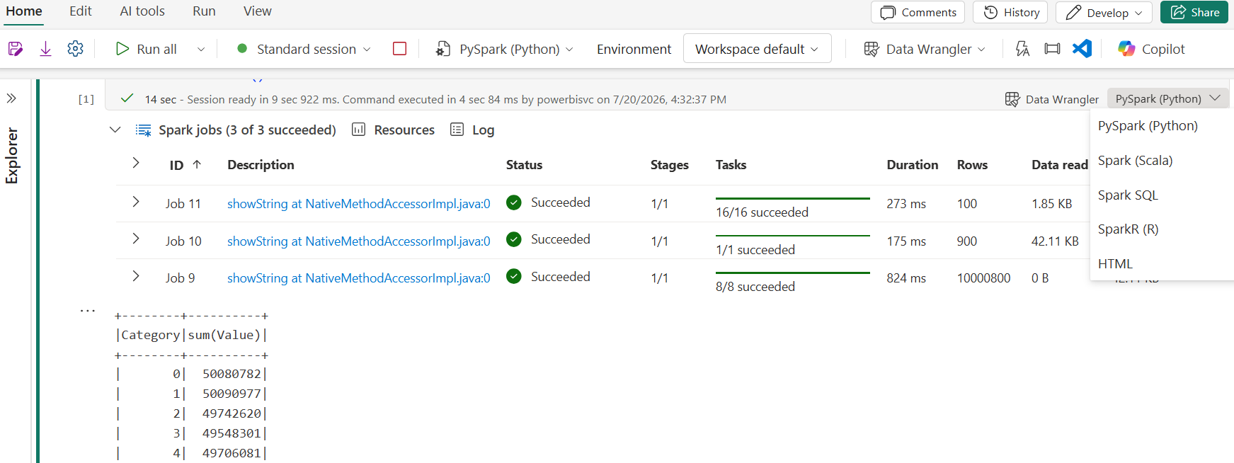
After migration work on a large enterprise tenant, post-migration validation was more time-consuming than the migration itself. The Spark UI is the most underused tool in a Fabric engineer’s workflow — specifically the Stages tab, which shows shuffle volume per stage. If your shuffle read is more than ten times your input data size, you have a join or aggregation problem that no amount of SKU upgrades will fix.

Section 04

Orchestration & Scheduling

Notebooks are not self-scheduling. You cannot put a cron expression in a notebook and call it done. Production scheduling in Fabric is handled exclusively by Data Pipelines — the Notebook activity within a pipeline is what gives a notebook its schedule, retry logic, timeout, and monitoring.

Step 1 — Parameterize the Notebook

A notebook that cannot accept external parameters is only suitable for interactive development. Before adding it to a pipeline, parameterize every value that may vary between runs.

PySpark — runtime parameters via mssparkutils

from datetime import datetime, timedelta

# Receive parameters from pipeline — fall back to sensible defaults
RUN_DATE    = mssparkutils.runtime.getParameterValue(
    "run_date", str((datetime.now() - timedelta(days=1)).date()))
ENVIRONMENT = mssparkutils.runtime.getParameterValue("environment", "prod")

CURATED_TABLE = (
    "curated.sales" if ENVIRONMENT == "prod" else "curated_dev.sales"
)

print(f"run_date={RUN_DATE} | env={ENVIRONMENT} | target={CURATED_TABLE}")

Step 2 — Add the Notebook to a Pipeline

Create a Data PipelineIn your workspace, click + New item → Data pipeline. Give it a clear name: daily_sales_etl, not pipeline_1.
Add a Notebook ActivityDrag Notebook from the Activities panel onto the canvas. In the Settings tab, select your notebook. Under Base parameters, map pipeline variables to the notebook parameters (run_date, environment).
Configure Retry and TimeoutSet retry count to 2 with a 5-minute delay. Set timeout to match your SLA window — a daily job with a 2-hour window should timeout at 90 minutes, not 24 hours.
Add Failure HandlingConnect a failure branch to a notification activity (email or Teams webhook). A pipeline that silently fails is worse than one that never runs.
Schedule the PipelineClick Schedule in the ribbon. Set recurrence. The schedule lives on the pipeline, not the notebook — the notebook itself has no schedule awareness.

Step 3 — Git Integration and CI/CD

Project structure — Git repository layout

fabric-data-engineering/
├── notebooks/
│   ├── sales_transform.py          # Daily sales ETL
│   ├── customer_features.py        # ML feature engineering
│   └── table_maintenance.py        # OPTIMIZE + VACUUM runner
├── tests/
│   ├── test_sales_schema.py
│   └── test_merge_idempotency.py
├── configs/
│   └── pipeline_params_prod.json
└── README.md

ℹ️

Git Sync — Workspace Branches

Fabric workspaces support branch-per-environment CI/CD. The main branch connects to Production, dev to Development. Promotion between environments uses deployment pipelines, not manual copy-paste.

Section 05

Security & Governance

Notebooks inherit permissions from the identity that runs them — your Entra ID in interactive sessions, the workspace identity or service principal in pipeline-scheduled runs. This distinction matters for production: always test pipeline runs under the same identity the pipeline will use.

Three-Layer Access Control

Layer	Mechanism	Practical Example
Workspace	Admin / Member / Contributor / Viewer roles	Engineers are Members. Analysts are Viewers — they can read reports but cannot edit notebooks.
Lakehouse	Row-level security (RLS) + column masking	Regional managers see only their region’s rows. Credit card numbers are masked for all non-finance roles.
Execution	Entra ID (interactive) or Service Principal (pipeline)	Pipeline runs as a service principal with read-only access to the raw zone and write access to the curated zone only.

PII Masking in Notebooks

PySpark — PII masking before writing to curated zone

from pyspark.sql.functions import col, when, substring, hash, concat, lit

# Mask national ID — retain last 4 digits only
df_masked = df.withColumn(
    "national_id_masked",
    when(col("national_id").isNotNull(),
         concat(lit("XXX-XX-"), substring(col("national_id"), 8, 4)))
    .otherwise(None)).drop("national_id")

# Hash email for join compatibility without exposing PII
df_masked = df_masked.withColumn(
    "email_hash", hash(col("email"))).drop("email")

# Assert no PII leaked before writing
pii_cols = ["national_id", "email", "phone", "credit_card"]
leaked = [c for c in df_masked.columns if c in pii_cols]
assert len(leaked) == 0, f"PII leak detected: {leaked}"

df_masked.write.format("delta").mode("append").saveAsTable("curated.customers_masked")

✅

Microsoft Purview Integration

Microsoft Purview scans Fabric Lakehouses automatically when connected to the workspace. Notebook-to-table lineage is captured without any additional configuration — every write from a notebook to a Delta table appears in the Purview data catalog with full column-level lineage. Enable Purview integration in Fabric Admin Portal → Governance settings.

Section 06

Production Recipes

Complete, copy-ready notebooks for the three most common production scenarios. Each recipe follows all five patterns from Section 02.

Recipe 1 — Daily Sales ETL with Quality Gate

PySpark — full daily ETL notebook

# ============================================================
# NOTEBOOK: sales_daily_etl
# INPUTS:   Raw CSV in ADLS Gen2 — abfss://raw/.../sales/{date}/
# OUTPUTS:  curated.sales (Delta — upserted)
#           errors.sales_quality (Delta — appended)
# RUNS:     Daily @ 02:00 UTC via Data Pipeline "daily_sales_etl"
# OWNER:    data-engineering@company.com
# ============================================================

from datetime import datetime, timedelta
from pyspark.sql.functions import col, current_timestamp, lit, when
from delta.tables import DeltaTable

RUN_DATE = mssparkutils.runtime.getParameterValue(
    "run_date", str((datetime.now() - timedelta(days=1)).date()))
SOURCE = f"abfss://raw@{STORAGE}.dfs.core.windows.net/sales/{RUN_DATE}/"

print(f"Starting daily ETL for {RUN_DATE}")

# 1. READ
df_raw = spark.read.option("header", "true").csv(SOURCE)
print(f"Read {df_raw.count():,} raw rows")

# 2. QUALITY GATE
bad = df_raw.filter(col("order_id").isNull() | (col("amount") < 0))
if bad.count() > 0:
    (bad.withColumn("captured_at", current_timestamp())
       .write.format("delta").mode("append")
       .saveAsTable("errors.sales_quality"))

# 3. CLEAN
df_clean = (df_raw
    .filter(col("order_id").isNotNull() & (col("amount") >= 0))
    .dropDuplicates(["order_id"])
    .withColumn("ingestion_ts", current_timestamp())
    .withColumn("run_date", lit(RUN_DATE)))

# 4. MERGE (idempotent)
target = DeltaTable.forName(spark, "curated.sales")
(target.alias("tgt")
    .merge(df_clean.alias("src"), "tgt.order_id = src.order_id")
    .whenMatchedUpdateAll()
    .whenNotMatchedInsertAll()
    .execute())

print(f"✅ ETL complete: {df_clean.count():,} rows merged")

Recipe 2 — Hourly KPI Refresh for Power BI

PySpark — rolling KPI aggregation

from pyspark.sql.functions import sum, count, avg, current_date, current_timestamp, col
from delta.tables import DeltaTable

# Rolling 30-day window — avoids full historical scan
sales = (spark.read.format("delta").table("curated.sales")
    .filter(col("sale_date") >= current_date() - 30))

kpi = (sales
    .groupBy("sale_date", "region")
    .agg(
        sum("amount").alias("daily_revenue"),
        count("*").alias("order_count"),
        avg("amount").alias("avg_order_value"))
    .withColumn("refreshed_at", current_timestamp()))

target = DeltaTable.forName(spark, "reporting.kpi_daily")
(target.alias("tgt")
    .merge(kpi.alias("src"),
        "tgt.sale_date = src.sale_date AND tgt.region = src.region")
    .whenMatchedUpdateAll()
    .whenNotMatchedInsertAll()
    .execute())

print(f"✅ KPI table refreshed: {kpi.count():,} region-date combinations")

Section 07

Notebooks vs. Alternatives

The correct tool depends on data volume, logic complexity, and team skillset. There is no universal answer — but there are clear wrong answers for specific scenarios.

Scenario	Right Tool	Wrong Tool	Why
Daily 10 GB CSV → Delta merge	Notebook	Dataflow Gen2	Dataflow costs ~10× more at this scale. Notebooks handle it in minutes.
Simple lookup join for BI analysts	SQL Warehouse	Notebook	SQL Warehouse has lower latency for ad-hoc analytical queries on structured data.
Visual mapping from Excel for a business user	Dataflow Gen2	Notebook	Dataflows are low-code. Asking a business user to write PySpark is the wrong trade-off.
ML feature engineering (100 GB+)	Notebook	SQL Warehouse	Notebooks integrate with scikit-learn, MLflow, and Fabric ML. SQL Warehouse does not.
Real-time streaming transformation	Notebook (Structured Streaming)	Dataflow Gen2	Dataflows are batch. Notebooks support Spark Structured Streaming for low-latency pipelines.
Complex multi-source join with custom logic	Notebook	SQL Warehouse	PySpark supports arbitrarily complex logic, UDFs, and Python libraries that SQL cannot.

Dataflow Gen2 and SQL Warehouse are not inferior tools — they are the right tools for specific jobs. Notebooks win on cost and flexibility for large-scale, complex, or ML-adjacent transformations.

📌

Cost Context — Notebooks vs. Dataflow Gen2

The 90% cost savings figure cited by the community applies specifically to large-scale transformations (10 GB+) where Dataflow Gen2’s per-row execution model becomes expensive. For small datasets under 1 GB processed infrequently, the cost difference is negligible. Size the tool to the workload, not the other way around. Ensure your notebooks are correctly paused by following our Fabric capacity optimization guide.

Section 08

Frequently Asked Questions

Do I need a Pro licence to run notebooks in Fabric?

No. Fabric notebooks run on F-SKU capacity (minimum F2) — there is no per-user Pro licence requirement for data engineers who create and run notebooks. Viewers of content published from notebooks to Power BI reports may still need a Pro licence below F64 capacity, but the notebook itself does not require one.

Why does my notebook have a 20–60 second cold start?

Cold start is the time it takes for the Spark cluster to initialize when a new session begins. On F2–F4 capacities, cold start is typically 20–60 seconds. On F8 and above, it is usually under 20 seconds. Once the session is running, subsequent cells execute immediately. In pipeline runs, schedule notebooks to run back-to-back in the same pipeline where possible to avoid repeated cold starts.

How do I read from a Lakehouse in a different workspace?

Two options. First, create a OneLake shortcut in your Lakehouse pointing to the target table in the other workspace — it then appears as a local table. Second, use the full abfss:// path directly in your notebook:

spark.read.format("delta").load("abfss://workspace@onelake.dfs.fabric.microsoft.com/lakehouse.Lakehouse/Tables/table_name")

. The shortcut approach is cleaner for ongoing pipelines.

My notebook produces duplicate rows on rerun. How do I fix it?

You are using .write.mode("append") without deduplication, or the notebook runs multiple times for the same data window. The fix is to replace append writes with Delta MERGE keyed on a business identifier (order ID, customer ID, etc.). MERGE is idempotent — running it ten times on the same input produces the same result.

Can I use Python libraries not included in the default Fabric runtime?

Yes. Install libraries inline using %pip install library_name in a notebook cell — this installs to the current session only. For persistent installation across all notebooks in a workspace, use the Workspace library management settings (Environment item → Libraries tab).

How do I schedule a notebook to run daily?

Notebooks do not have their own scheduling — scheduling is handled exclusively by Data Pipelines. Create a pipeline, add a Notebook activity, and schedule the pipeline. The notebook receives parameters via the activity’s Base parameters setting. Do not use the notebook’s own “Schedule” button for production — it runs the notebook directly without retry logic, timeout, or downstream failure handling.

What is the difference between OPTIMIZE and VACUUM?

OPTIMIZE compacts small Delta files into larger ones, improving read performance. It is safe to run at any time — readers continue working uninterrupted. VACUUM deletes old Delta file versions that fall outside the retention window (default 7 days). VACUUM is destructive — once old versions are removed, time travel to those snapshots is no longer possible. Run VACUUM during maintenance windows, not while active queries are running.

⚠ Accuracy Disclaimer

Code examples and feature descriptions are based on the Microsoft Fabric Spark 3.5 runtime and official Microsoft documentation at time of writing (June 2026). API behaviour and available features change with runtime updates — always verify against learn.microsoft.com/fabric/data-engineering/runtime before deploying to production. UIG Data Lab is an independent publication, not affiliated with or endorsed by Microsoft Corporation.

A.J. Data Engineering Researcher & Technical Writer · UIG Data Lab All articles →

A.J. researches and writes about data engineering, analytics architecture, Microsoft Fabric, and modern cloud data platforms. Coverage spans Microsoft Fabric, Power BI, Azure Data Engineering, Databricks, Snowflake, Apache Spark, dbt, Apache Airflow, and modern cloud data infrastructure. The focus is practitioner-level content that helps data professionals understand platform capabilities, evaluate technology decisions, optimize costs, and implement practical solutions using official documentation, product updates, community insights, and industry best practices. His writing covers real decisions from real deployments — not documentation rewrites.

Microsoft Fabric Real-Time Intelligence KQL Databricks Apache Spark dbt Azure Synapse Snowflake AWS Data Architecture

Transform Data Using Notebooks in Microsoft Fabric

Executive Summary – Transform Data Using Notebooks

Setup & First Run

Prerequisites

Create and Attach a Notebook

Five Production Patterns

Pattern 1 — Schema Enforcement and Quality Gates

Pattern 2 — Idempotent Merges with Delta MERGE

Pattern 3 — Window Functions for Time-Series Features

Pattern 4 — Incremental Ingestion with Partition Pruning

Pattern 5 — Feature Engineering for ML

Performance Optimization

Partition by Date or Business Key

Broadcast Small Dimension Tables

Filter Before Joins

V-Order and Liquid Clustering

Shuffle Partition Tuning

OPTIMIZE and VACUUM

Orchestration & Scheduling

Step 1 — Parameterize the Notebook

Step 2 — Add the Notebook to a Pipeline

Step 3 — Git Integration and CI/CD

Security & Governance

Three-Layer Access Control

PII Masking in Notebooks

Production Recipes

Recipe 1 — Daily Sales ETL with Quality Gate

Recipe 2 — Hourly KPI Refresh for Power BI

Notebooks vs. Alternatives

Frequently Asked Questions

Related Posts